Regression Indicator Variable With and Added Continuous Measure
Does sex influence confidence in the police?
We want to perform linear regression of the police confidence score against sex, which is a binary categorical variable with two possible values (which we can see are 1= Male and 2= Female if we check the Values cell in the sex row in Variable View). However, before we begin our linear regression, we need to recode the values of Male and Female. Why must we do this?
The codes 1 and 2 are assigned to each gender simply to represent which distinct place each category occupies in the variable sex. However, linear regression assumes that the numerical amounts in all independent, or explanatory, variables are meaningful data points. So, if we were to enter the variable sex into a linear regression model, the coded values of the two gender categories would be interpreted as the numerical values of each category. This would provide us with results that would not make sense, because for example, the sex Female does not have a value of 2.
We can avoid this error in analysis by creating dummy variables.
Dummy Variables
A dummy variable is a variable created to assign numerical value to levels of categorical variables. Each dummy variable represents one category of the explanatory variable and is coded with 1 if the case falls in that category and with 0 if not. For example, in the dummy variable for Female, all cases in which the respondent is female are coded as 1 and all other cases, in which the respondent is Male, are coded as 0. This allows us to enter in the sex values as numerical. (Remember, these numbers are just indicators.)
Because our sex variable only has two categories, turning it into a dummy variable is as simple as recoding the values of Male and Female from 1=Male and 2=Female to 0=Male and 1=Female. (We will see later that creating dummy variables for categorical variables with multiple levels takes just a little more work.) However, it's good practice to create a new variable altogether when you are creating dummy variables. This way, if you make an error while building the dummy variables, you haven't altered your original variable and can always start again.
To begin, select Transform and Recode into Different Variables.
Find our variable sex in the variable list on the left and move it to the Numeric Variable -> Output Variable text box.
Next, under the Output Variable header on the left, enter in the name and label for the new sex variable we're creating. We've chosen to call this new variable sex1 and label it Sex Dummy Variable.
Click Change, to move your new output variable into the Numeric Variable -> Output Variable text box in the centre of the dialogue box.
Then, select Old and New Values.
Enter 1 under the Old Value header and 0 under the New Value header. Click Add. You should see 1 -> 0 in the Old -> New text box. Now enter 2 under the Old Value header and 1 under the New Value header. Click Add, and then Continue.
Finally, click OK in the original Recode into Different Variables dialogue box. Scroll down to the very end of the variables list in Variable View. You should see your new dummy variable sex1 at the end of the list, as it's the last variable to be created.
Now, let's run our first linear regression, exploring the relationship between policeconf1 and sex1.
To perform simple linear regression, select Analyze, Regression, and Linear…
Find policeconf1 in the variable list on the left and move it to the Dependent box at the top of the dialogue box. Find sex1 in the variable list and move it to the Independent(s) box in the centre of the dialogue box. Click OK.
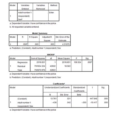
Your output should look like that output tables on the right.

For our purposes, you don't need to be concerned with most of the results above – you can learn more about these as you become more experienced. However, from some of these, we can work out the effect of sex on confidence in the police.
We can use our SPSS results to write out the fitted regression equation for this model and use it to predict values of police confidence for given certain values of sex.
Using the output from SPSS, we can calculate the mean confidence in the police for men and women using the following regression equation:
Y = a + bX
where Y is equal to our dependent variable and X is equal to our independent variable.
Into this equation, we will substitute a and b with the statistics provided in the Coefficients output table, a being the constant coefficient and b being the coefficient associated with sex (our explanatory variable).
In this example, our equation should look like this:
policeconf1 = 13.761 + (-0.436 x sex)
Since sex takes on the value of 1 for female and 0 for male, the predicted scores are as follows:
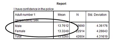
policeconf1 = 13.761 + (-0.436 x 1) = 13.325 (Females)
policeconf1 = 13.761 + (-0.436 x 0) = 13.761 (Males)
So, on average, female respondents reported a police confidence score that is .436 points lower than male respondents.
Think about how policeconf1 is measured. In this variable, what does a lower score mean? Also, if you've been following all the analyses we've done in this section, these scores may look familiar to you. Consider where you might have seen these scores before.
Rather than just accepting these results, we now want to gauge how much of the variation in policeconf1 is explained by sex1. To do this we can simply use the r2 statistic which you will find is already calculated for you in the Model summary output table above. In this example, the r2 is very low at 0.003. This shows that only 0.3% of the variation in police confidence is explained by sex (0.003 x 100 to give us a percentage). This suggests that there are many other factors that might be affecting a respondent's confidence in the police.
The linear regression model above allowed us to calculate the mean police confidence scores for men and women in our dataset. We can check to see if our calculated mean scores are correct by using the Compare Means function of SPSS (Analyze, Compare Means, Means, with policeconf1 as the Dependent variable and sex as the Independent variable).

What are the results of your mean comparison? They should be exactly the same as the means we calculated above. Calculating the mean scores using simple linear regression, with just one independent variable, was effectively the same function as comparing the means. As we'll see later, multiple linear regression allows the means of many variables to be considered and compared at the same time, while reporting on the significance of the differences.
Determining the Significance of the Independent Variable
What is the significance of sex as a predictor of police confidence score?
Our sample of data has shown us that, on average, female respondents reported a police confidence score that is .436 points lower than male respondents. We want to know if this is a statistically significant effect in the population from which the sample was taken. To do this, we carry out a hypothesis test to determine whether or not b (the coefficient for females) is different from zero in the population. If the coefficient could be zero, then there is no statistically significant difference between males and females.
SPSS calculates a t statistic and a corresponding p-value for each of the coefficients in the model. These can be seen in the Coefficients output table. A t statistic is a measure of how likely it is that the coefficient is not equal to zero. It is calculated by dividing the coefficient by the standard error. If the standard error is small relative to the coefficient (making the t statistic relatively large), the coefficient is likely to differ from zero in the population.
The p-value is in the column labelled Sig. As in all hypothesis tests, if the p-value is less than 0.05, then the variable is significant at the 5% level. That is, we would have evidence to reject the null and conclude that b is different from zero.
In this example, t = -10.417 with a corresponding p-value of 0.000. This means that the chances of the difference between males and females that we have calculated is actually happening due to chance is very small indeed. Therefore, we have evidence to conclude that sex1 is a significant predictor of policeconf1 in the population.
Summary
You've just used linear regression to study the relationship between our continuous dependent variable policeconf1 and sex, a categorical independent variable with just two categories. Using linear regression, you were able to predict police confidence scores for men and women. What if you wanted to fit a linear regression model using police confidence score and something like ethnicity, a categorical independent variable with more than two categories? The next page will take you through how to run a simple linear regression with a categorical independent variable with several categories.
Note: as we are making changes to a dataset we'll continue using for the rest of this section, please make sure to save your changes before you close down SPSS. This will save you having to repeat sections you've already completed.
Source: https://www.southampton.ac.uk/passs/confidence_in_the_police/multivariate_analysis/linear_regression.page
0 Response to "Regression Indicator Variable With and Added Continuous Measure"
Post a Comment